Sections
General
In StructuralCodes, a Section is responsible for connecting a geometry object with an API for performing calculations on the geometry.
The section contains a SectionCalculator which contains the API for doing calculations on the geometry, including for example lower level methods for integrating a strain profile to stress resultants, or calculating a strain profile based on stress resultants, or higher level methods like calculating a moment-curvature relation, or an interaction diagram between moments and axial force.
The SectionCalculator uses a SectionIntegrator to integrate the strain response on a geometry.
Tip
See the theory reference for a guide on the sign convention used in StructuralCodes.
Tip
The theory reference provides an overview of the theory behind the section calculator and the section integrators.
The beam section
The BeamSection takes a SurfaceGeometry or a CompoundGeometry as input, and is capable of calculating the response of an arbitrarily shaped geometry with arbitrary reinforcement layout, subject to stresses in the direction of the beam axis.
In the example below, we continue the example with the T-shaped geometry.
Tip
If you are looking for the gross properties of the section, these are available at the .gross_properties property on the Section object ✅
Since the axial force and the moments are all relative to the origin, we start by translating the geometry such that the centroid is alligned with the origin.
Notice how we can use .calculate_bending_strength() and .calculate_limit_axial_load() to calculate the bending strength and the limit axial loads in tension and compression.
Furthermore, we have the following methods:
.integrate_strain_profile()Calculate the stress resultants for a given strain profile.
.calculate_strain_profile()Calculate the strain profile for given stress resultants.
.calculate_moment_curvature()Calculate the moment-curvature relation.
.calculate_nm_interaction_domain()Calculate the interaction domain between axial load and bending moment.
.calculate_nmm_interaction_domain()Calculate the interaction domain between axial load and biaxial bending.
.calculate_mm_interaction_domain()Calculate the interaction domain between biaxial bending for a given axial load.
See the BeamSectionCalculator for a complete list.
Note
Notice that a call to .calculate_nm_interaction_domain() returns the interaction domain for a negative bending moment, i.e. a bending moment that gives compression at the top of the cross section according to the sign convention. To obtain the interaction domain for the positive bending moment, the neutral axis for the calculation should be rotated an angle \(\theta = \pi\), i.e. the method should be called with the keyword argument theta = np.pi or theta = math.pi. Alternatively, to return the complete domain, the method could be called with the keyword argument complete_domain = True.
Syntax
from structuralcodes.sections import BeamSection

# Create a section
section_not_translated = BeamSection(geometry=t_geom)

# Use the centroid of the section, given in the gross properties, to re-allign
# the geometry with the origin
t_geom = t_geom.translate(dy=-section_not_translated.gross_properties.cz)
section = BeamSection(geometry=t_geom)

# Calculate the bending strength
bending_strength = section.section_calculator.calculate_bending_strength()

# Calculate the limit axial loads
limit_axial_loads = section.section_calculator.calculate_limit_axial_load()

# Calculate the interaction domain between axial force and bending moment
nm = section.section_calculator.calculate_nm_interaction_domain()

# Calculate the moment-curvature relation
moment_curvature = section.section_calculator.calculate_moment_curvature()
Notice how for example .calculate_moment_curvature() returns a custom dataclass of type MomentCurvatureResults. If we inspect this class further, we find among its attributes chi_y and m_y. These are the curvature and the moment about the selected global axis of the section. We also find the curvature and moment about the axis orthogonal to the global axis chi_z and m_z, and the axial strain at the level of the global axis eps_axial. All these attributes are stored as arrays, ready for visualization or further processing.
Tip
Use your favourite plotting library to visualize the results from the BeamSectionCalculator. The code below shows how to plot the moment-curvature relation in the figure below with Matplotlib. Notice how we are plotting the negative values of the curvatures and moments due to the sign convention.
Syntax
import matplotlib.pyplot as plt

# Visualize moment-curvature relation
fig_momcurv, ax_momcurv = plt.subplots()
ax_momcurv.plot(
    -moment_curvature.chi_y * 1e3, -moment_curvature.m_y * 1e-6, '-k'
)
ax_momcurv.grid()
ax_momcurv.set_xlabel(r'$\chi_{\mathrm{y}}$ [1/m]')
ax_momcurv.set_ylabel(r'$M_{\mathrm{y}}$ [kNm]')
ax_momcurv.set_xlim(xmin=0)
ax_momcurv.set_ylim(ymin=0)
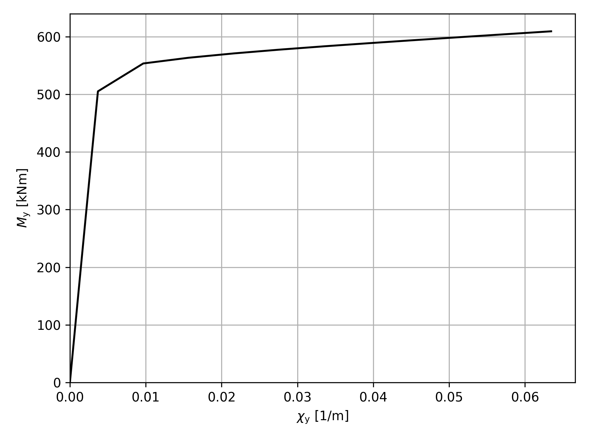
The moment-curvature relation computed with the code above.
Inspecting further with results objects
The results objects contain methods for inspecting and processing further the detailed results on the section after a calculation is performed.
For instance, calling the method .calculate_bending_strength() returns an object of class UltimateBendingMomentResults.
The object contains the following methods:
.create_detailed_result()Create an object of class
SectionDetailedResultStatewith the datastructure storing strain and stress fields across the section..get_point_strain()Get the strain at a point.
.get_point_stress()Get the stress at a point.
In the example below, we continue the example with the T-shaped geometry and we create the detailed_result.
Syntax
# Calculate the bending strength
bending_strength = section.section_calculator.calculate_bending_strength()
# Create the detailed_results data structure
bending_strength.create_detailed_result(num_points=10000)
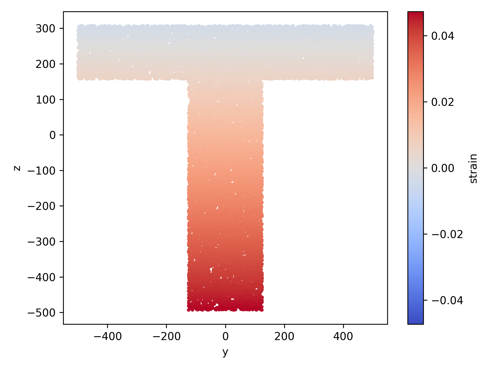
If we inspect this result object, we find among its attributes detailed_result that has two useful datastructures: one for surface geometries and one for point geometries. The datastructure for surface geometries contains all points samples from the geometries. These data structures can be easily input for creating a DataFrame object permitting further processing. For instance in the example below, we use pandas plotting abilities to create a visualization of strain and stress fields.
Syntax
# Visualize bending strength strain field
df = pd.DataFrame(bending_strength.detailed_result.surface_data)
fig_strain, ax_strain = plt.subplots()
norm = mcolors.CenteredNorm(vcenter=0)
abs_max = df['strain'].abs().max()
df.plot.scatter(
x='y', y='z', s=5, c='strain', ax=ax_strain, cmap='PiYG', norm=norm
)
fig_strain.tight_layout()
fig_strain.savefig('strain_field.png', dpi=300)
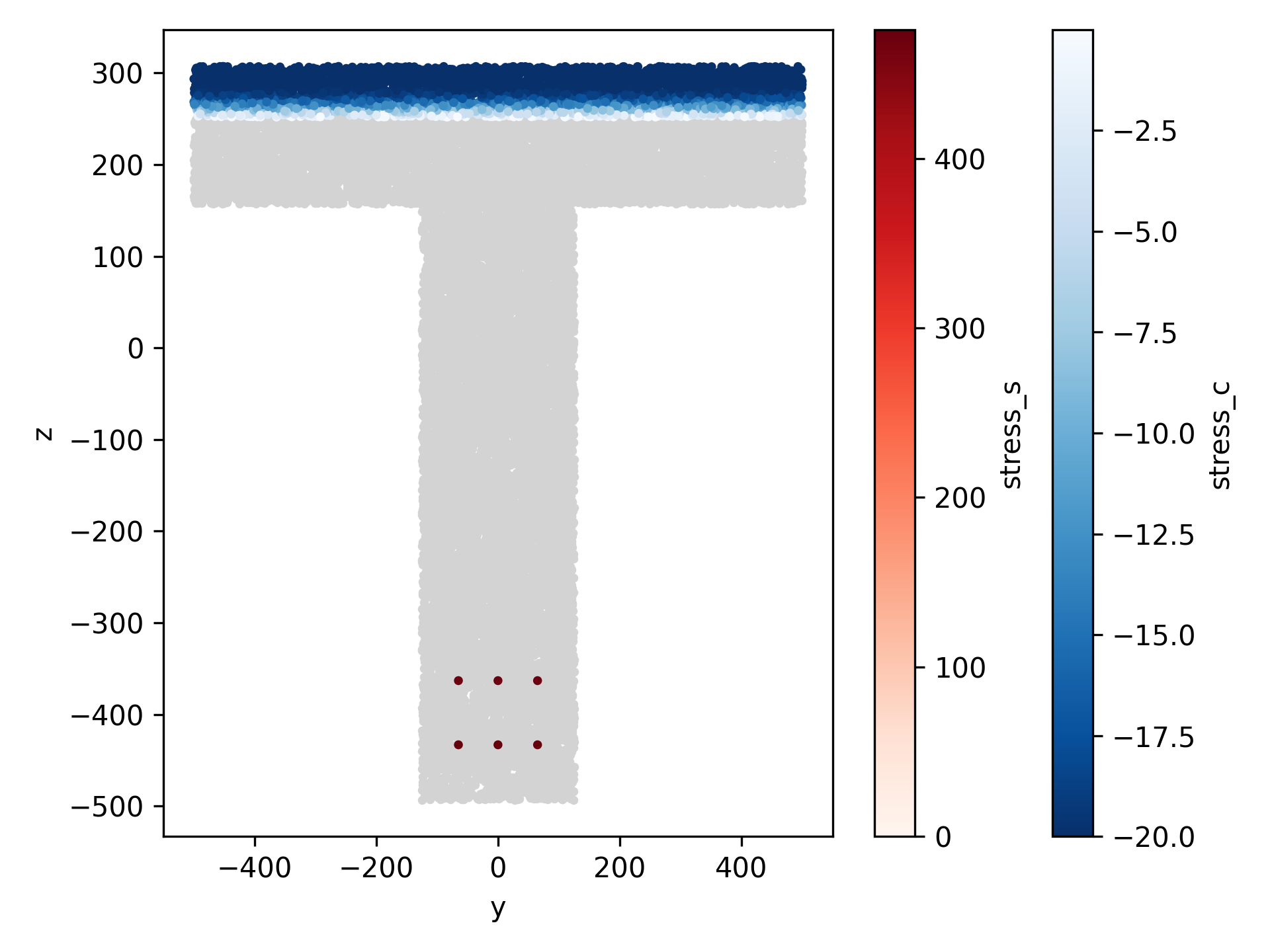
# Visualize bending strength stress field
df_p = pd.DataFrame(bending_strength.detailed_result.point_data)
fig_stress, ax_stress = plt.subplots()
# plot as background all concrete fibers in grey
df.plot.scatter(x='y', y='z', s=5, color='lightgray', zorder=1, ax=ax_stress)
# Plot compressed concrete fibers
# Rename just to have a nicer label. Alternative is plotting manually with
# matplotlib and controlling the colorbar
df.rename(columns={'stress': 'stress_c'}).query('stress_c < 0.0').plot.scatter(
x='y', y='z', s=5, c='stress_c', cmap='Oranges_r', zorder=2, ax=ax_stress
)
# Plot reinforcement fibers
# Rename just to have a nicer label. Alternative is plotting manually with
# matplotlib and controlling the colorbar
df_p.rename(columns={'stress': 'stress_s'}).plot.scatter(
x='y',
y='z',
s=5,
c='stress_s',
cmap='Blues',
zorder=3,
ax=ax_stress,
vmin=0,
)
fig_stress.tight_layout()
fig_stress.savefig('stress_field.png', dpi=300)
If we only want to know the strain and/or stress at a specific point we can directly use methods .get_point_strain() or .get_point_stress() without the need of creating the detailed result. For instance with the code below we query the stress at a point for any geometry whose group_label matches the pattern "reinforcement". Note that a pattern can be given with wildcards (like '*' or '?'); for more information refer to .get_point_stress() and .group_filter().
Syntax
# Get the stress at a specific point in the section
coord_reinf = (
    section.geometry.point_geometries[0].x,
    section.geometry.point_geometries[0].y,
)
stress = bending_strength.get_point_stress(
    *coord_reinf, group_label='reinforcement'
)
print(f'Stress at point {coord_reinf}: {stress:.2f} MPa')
When dealing with analysis that do not involve a single section state, like for instance a Moment-Curvature analysis, the detailed_result object is created for the current_step. The current_step is initialized at 0. Then methods are available for navigating through steps:
.next_step()Navigate to the next step.
.previous_step()Navigate to the previous step.
.set_step()Navigate to a specific step.
If we are not interested in getting the detailed results but we want to get the stresses and/or strains at specific points the same methods .get_point_stress() and .get_point_strain() can be used. In this case the return will be an array of stresses (or strains) for the point through the moment-curvature analysis. For instance with the code below it is possible to plot the stress for one rebar at a given position for the increasing curvature.
Syntax
# Plot the stress at rebar for increasing curvature
# Get the stress at a specific point in the section
coord_reinf = (
    section.geometry.point_geometries[0].x,
    section.geometry.point_geometries[0].y,
)
stress = moment_curvature.get_point_stress(
    *coord_reinf, group_label='reinforcement'
)

fig_stress_mc, ax_stress_mc = plt.subplots()
ax_stress_mc.plot(
    -moment_curvature.chi_y,
    stress,
    '-k',
    label=f'Stress at point ({coord_reinf[0]:.0f}, {coord_reinf[1]:.0f}),',
)
ax_stress_mc.set_xlabel(r'$\chi_y$')
ax_stress_mc.set_ylabel('Stress [MPa]')
ax_stress_mc.grid(True)
ax_stress_mc.legend()
ax_stress_mc.set_xlim(xmin=0)
ax_stress_mc.set_ylim(ymin=0)
fig_stress_mc.tight_layout()
fig_stress_mc.savefig('stress_at_rebar.png', dpi=300)
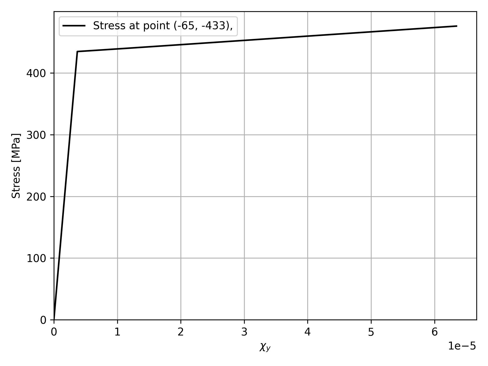
The stress for increasing curvature plotted with the code above.
Using in a more advanced way matplotlib, it is possible to create an animation (like for instance a gif file) showing the stress field for the steps of the moment-curvature analysis. The code below create an animation with the moment curvature diagram on the left and the cross section stress field on the right.
Syntax
# Create a gif animation of stress field
chi = -moment_curvature.chi_y
mom = -moment_curvature.m_y * 1e-6  # kNm
n_steps = len(chi)

# Precompute axis limits and color limits to avoid jumping during animation
# Section limits from one representative detailed result
moment_curvature.set_step(0)
df0 = pd.DataFrame(moment_curvature.detailed_result.surface_data)
df0_p = pd.DataFrame(moment_curvature.detailed_result.point_data)
ymin = df0['y'].min()
ymax = df0['y'].max()
zmin = df0['z'].min()
zmax = df0['z'].max()
dy = ymax - ymin
dz = zmax - zmin
pad_y = 0.05 * dy if dy > 0 else 1.0
pad_z = 0.05 * dz if dz > 0 else 1.0
# Precompute stress ranges over all steps so the colormap stays fixed
concrete_min = 0.0
steel_max = 0.0

for i in range(n_steps):
    moment_curvature.set_step(i)
    c_min = np.asarray(
        moment_curvature.detailed_result.surface_data['stress']
    ).min()
    concrete_min = min(concrete_min, c_min)
    s_max = np.asarray(
        moment_curvature.detailed_result.point_data['stress']
    ).max()
    steel_max = max(steel_max, s_max)

# Create figure and fixed artists
fig, (ax_mc, ax_sec) = plt.subplots(1, 2, figsize=(14, 6))
# ---- Left: moment-curvature curve
ax_mc.plot(chi, mom, '-k', lw=1.5)
(point_mc,) = ax_mc.plot([], [], 'or', ms=6)

ax_mc.set_xlabel(r'$\chi_y$')
ax_mc.set_ylabel(r'$M_y$ [kNm]')
ax_mc.grid(True)
ax_mc.set_xlim(xmin=0)
ax_mc.set_ylim(ymin=0)

title_mc = ax_mc.set_title('Moment-curvature response')

# ---- Right: section stress field
ax_sec.set_xlabel('y')
ax_sec.set_ylabel('z')
ax_sec.set_aspect('equal')
ax_sec.grid(True)
ax_sec.set_xlim(ymin - pad_y, ymax + pad_y)
ax_sec.set_ylim(zmin - pad_z, zmax + pad_z)

title_sec = ax_sec.set_title('Stress distribution')

# Create empty scatter artists once
ax_sec.scatter(df0['y'], df0['z'], s=4, c='lightgray', zorder=1)
sc_conc = ax_sec.scatter(
    [], [], s=5, c=[], cmap='Oranges_r', zorder=2, vmin=concrete_min, vmax=0.0
)
sc_steel = ax_sec.scatter(
    [], [], s=20, c=[], cmap='Blues', zorder=3, vmin=0.0, vmax=steel_max
)

# Optional colorbars
cbar_conc = fig.colorbar(sc_conc, ax=ax_sec)
cbar_conc.set_label('Concrete stress [MPa]')

cbar_steel = fig.colorbar(sc_steel, ax=ax_sec)
cbar_steel.set_label('Reinforcement stress [MPa]')


# Update function for animation
def update(frame):
    # Update analysis step
    moment_curvature.set_step(frame)
    dr = moment_curvature.detailed_result

    # ---- Left panel: moving point on M-k curve
    point_mc.set_data([chi[frame]], [mom[frame]])
    title_mc.set_text(
        f'Moment-curvature response - step {frame + 1}/{n_steps}'
    )

    # ---- Right panel: section plot
    # Compressed concrete only
    conc_offsets = np.column_stack(
        [np.asarray(dr.surface_data['y']), np.asarray(dr.surface_data['z'])]
    )
    conc_colors = np.asarray(dr.surface_data['stress'])
    conc_offsets = conc_offsets[conc_colors < 0, :]
    conc_colors = conc_colors[conc_colors < 0]

    sc_conc.set_offsets(conc_offsets)
    sc_conc.set_array(conc_colors)

    # Reinforcement fibers
    steel_offsets = np.column_stack(
        [np.asarray(dr.point_data['y']), np.asarray(dr.point_data['z'])]
    )
    steel_colors = np.asarray(dr.point_data['stress'])

    sc_steel.set_offsets(steel_offsets)
    sc_steel.set_array(steel_colors)

    title_sec.set_text(
        f'Stress distribution\n$\\chi_y$={chi[frame]:.4e},  $M_y$={mom[frame]:.2f} kNm'
    )

    return point_mc, sc_conc, sc_steel, title_mc, title_sec


# Build and save animation
fig.tight_layout()

anim = FuncAnimation(
    fig,
    update,
    frames=n_steps,
    interval=150,  # milliseconds between frames
    blit=False,  # safer with scatter + colorbars
    repeat=True,
)

anim.save(
    'moment_curvature_stress_animation.gif',
    writer=PillowWriter(fps=8),
    dpi=150,
)
The animation of the stress field with increasing curvature created with the code above.