Section integrators
The algorithms described in Section calculators require integration of stress or stiffness over the cross-section. This operation is performed using proper SectionIntegrator objects.
In StructuralCodes we have currently two distinct integrators: fiber integrator that discretize the cross section in a bunch of fibers (whose behavior is uniaxial), and marin integrator that is based on the computation of moments of area.
General concept
Section integrators compute properties such as stiffness, stress distribution, or strain compatibility over a section. They operate on the geometry and material definitions to derive these results.
Fiber integrator
This integrator uses a discretized approach where the section is divided into fibers, each representing a material point. This discretization is performed by a triangulation of the geometry. Each fiber is defined as the centre point of each triangle and is characterized by its competence area.
According to this integration, the integrals over the cross section are simply sums for all fibers. For instance, internal forces are determined as:
where \(\varepsilon_i\) is determined using equation (10) for each fiber:
Note
The triangulation is optimized in order to be executed only the first time a calculation on the section is performed. All fibers information (position \(y_i\), \(z_i\) and area \(A_i\)) are stored in numpy arrays. Therefore the application of (2) and of (1) is extremely fast making Fiber integrator the fastest integrator in StructuralCodes.
Marin integrator
Marin integrator implements the idea of prof. Joaquín Marín from University of Venezuela that he published during the ’80s [1].
The method performs an exact numerical solution of double integrals for polynomial functions acting over any plane polygonal surface (with or without holes) and is based on the computation of moments of area.
Within this context the moment of area of order \(m, n\) is described by the basic double integral:
where it is implicitly understood that \(\int_A ... \, dA\) represents a double integral.
If we consider a polynomial function with maximum exponents \(M\) and \(N\) respectivelly for \(y\) and \(z\), expressed in the following form, having indicated \(a_{m,n}\) any real coefficient for the term \(y^m z^n\):
the integral of the polynomial function over the cross-section, can be written as:
When the cross-section (i.e. the integration domain) is represented by a closed simply connected polygonal contour with \(P\) vertices, the moment of area of order \(m, n\) defined by (3) can be shown to be computed by the following relation:
where \(\binom{n}{k}\) indicates the usual binomial coefficients:
and (note that here we assume that \(P+1\) restarts from \(1\)):
Note
As mentioned, the integral is exact for polygonal surfaces and polynomial functions to be integrated over the surface.
If the cross-section is not polynomial, it must be discretized into a polygon (for instance a circular shape must be discretized as a polygon with \(P\) vertices) and therefore the integral is not exact anymore.
If the function to be integrated over the surface is not polynomial, the function can be discretized in linear branches and the cross section must be discretized in small polygons for each polynomial branch; also in this case the integral is not exact anymore.
The main application of this algorithm in StructuralCodes is for integrating the stress or modulus over the cross-section.
In this context, let’s consider a case of unixial bending, for which the stress function can be considered variable only with respect to coordinate \(z\):
In this case the internal forces \(N\), \(M_y\), \(M_z\) can be written as:
Hint
When the bending is not uniaxial anymore, one can consider the bidimensional normal stress polynomial:
An alternative approach is to rotate the section in order to have uniaxial bending in the new reference system \(y^*z^*\), see figure below. In StructuralCodes we are adopting the latter approach.
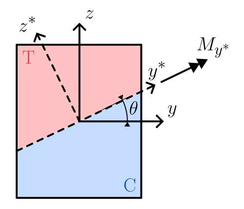
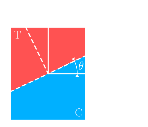
Rotation of reference system for having uniaxial bending.
The coeficients \(a_n\) are dependent on the stress function \(\sigma(z)\), therefore they depend on the constitutive law \(\sigma(\varepsilon)\). For this reason, each constitutive law that is used with Marin integration, must implement a special __marin__ method that returns the coefficients \(a_n\) for each polynomial branch that defines the constitutive law.
In determination of stiffness matrix, we need to integrate the tangent modulus over the cross-section. In this case we are integrating the function \(\sigma'\), where \(\cdot'\) indicates the derivative (i.e. the tangent modulus).
The determination of the coefficients for the constitutive laws implemented in StructuralCodes is reported in the following subsections.
Note
This means that if you write your custom constitutive law you must calculate the Marin coefficients for that law?
Don’t worry, we have done some work for you! Every material has a base version of __marin__ method, so you don’t have to implement it mandatorily. Keep in mind that the free __marin__ method works under a very simple idea: we linearize in several branches your law, obtaining a discretize piecewise constitutive law. For this discretized law we have the coefficients computed for the piece-wise linear law described below.
If your law can be represented (at least in branches) as polynomial functions it is way more efficient writing your custom __marin__ method since the integrator will split the polygon into as few as possible sub-polygons to perform the intergration.
So it is up to you! You can avoid bothering calculating and implementing Marin coefficients for stress and stiffness, but you can (and probably should) do it if you can optimize the calculation speed and if your constitutive law permits it.
Linear elastic material
The constitutive law of a linear elastic material can be written as:
For uniaxial bending the strain \(\varepsilon\) is equal to:
The stress function is easily obtained substituting (10) in (9):
Therefore the Marin coefficients \(a_n\) for linear elastic material are:
The stiffness is simply \(E\). Therefore:
And the only Marin coefficient is:
Elastic-plastic material
The constitutive law of an elastic plastic material with linear hardening is represented as in the figure below.
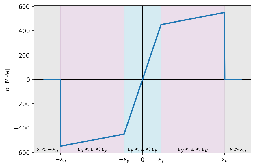
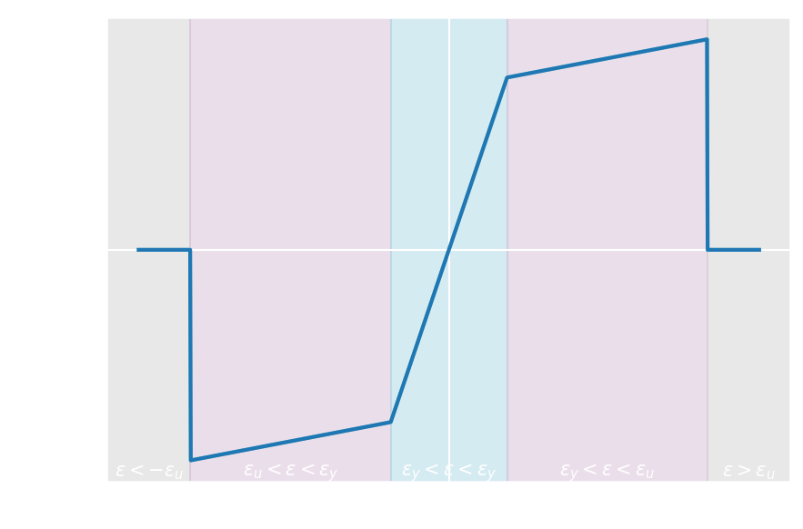
Elastic plastic with linear hardening law.
In this case, the constitutive law cannot be expressed as a whole with a single polynomial function, but looking at the picture above we can recognize 5 different portions, each one representing a different polynomial function. The constitutive law can then be written for the five branches as:
where \(E_h\) is the hardening modulus (i.e. the slope of the hardning branch) and \(\Delta \sigma = f_y \cdot \left(1 - \dfrac{E_h}{E}\right)\).
Substituting (10) in (15), one can compute the Marin coefficients for each branch. The coefficients are reported in the following table.
Branch name |
Strain range |
\(a_0\) |
\(a_1\) |
|---|---|---|---|
Elastic portion |
\(-\varepsilon_y < \varepsilon \le \varepsilon_y\) |
\(E \cdot \varepsilon_0\) |
\(E \cdot \chi_y\) |
Hardening (positive) |
\(\varepsilon_y < \varepsilon \le \varepsilon_u\) |
\(E_h \cdot \varepsilon_0 + \Delta \sigma\) |
\(E_h \cdot \chi_y\) |
Hardening (negative) |
\(-\varepsilon_u < \varepsilon \le -\varepsilon_y\) |
\(E_h \cdot \varepsilon_0 - \Delta \sigma\) |
\(E_h \cdot \chi_y\) |
Zero |
otherwise |
0.0 |
n.a. |
The __marin__ method returns the coefficients reported in the table above and the strain limits for each portion.
Then the integrator discretizes the polygon cutting it into the portions needed (depending on the strain distribution in the polygon) and for each subpolygon the exact Marin integration is performed.
The tangent stiffness can be represented by the following equation:
Therefore the marin coefficients for stiffness function are:
Branch name |
Strain range |
\(a_0\) |
|---|---|---|
Elastic portion |
\(-\varepsilon_y < \varepsilon \le \varepsilon_y\) |
\(E\) |
Hardening (positive) |
\(\varepsilon_y < \varepsilon \le \varepsilon_u\) |
\(E_h\) |
Hardening (negative) |
\(-\varepsilon_u < \varepsilon \le -\varepsilon_y\) |
\(E_h\) |
Zero |
otherwise |
0.0 |
Bilinear compression
The bilinear compression is characterized by no strength in tension and a linear behavior in compression up to \(\varepsilon_{c0}\) and then a constant stress equal to \(f_c\) (negative). After \(\varepsilon_{cu}\), the stress drops to 0. The constituive law is depicted the figure below.
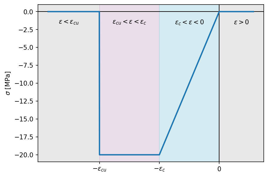
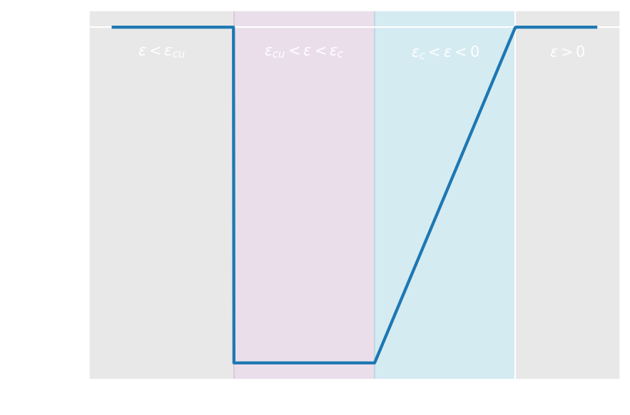
Bilinear compression constitutive law.
The constitutive law can be written in the following branches:
Substituting (10) in (17), one can compute the Marin coefficients for each branch. The coefficients are reported in the following table.
Branch name |
Strain range |
\(a_0\) |
\(a_1\) |
|---|---|---|---|
Elastic portion |
\(\varepsilon_{c0} \le \varepsilon < 0\) |
\(E \cdot \varepsilon_0\) |
\(E \cdot \chi_y\) |
Constant portion |
\(\varepsilon_{cu} \le \varepsilon < \varepsilon_{c0}\) |
\(f_c\) |
n.a. |
Zero |
otherwise |
0.0 |
n.a. |
The Marin coefficients for each branch for stiffness function are reported in the following table.
Branch name |
Strain range |
\(a_0\) |
|---|---|---|
Elastic portion |
\(\varepsilon_{c0} \le \varepsilon < 0\) |
\(E\) |
Constant portion |
\(\varepsilon_{cu} \le \varepsilon < \varepsilon_{c0}\) |
0.0 |
Zero |
otherwise |
0.0 |
Parabola rectangle
The parabola rectangle law, typically used for concrete, cannot be written as a whole with a polynomial law. Despite that, looking at the constitutive law plotted in the figure below, we can recognize a portion for the parabolic branch, a portion for the constant part and finally a portion for zero stress (both in tension and for excessive compression)
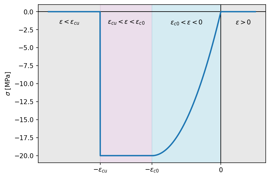
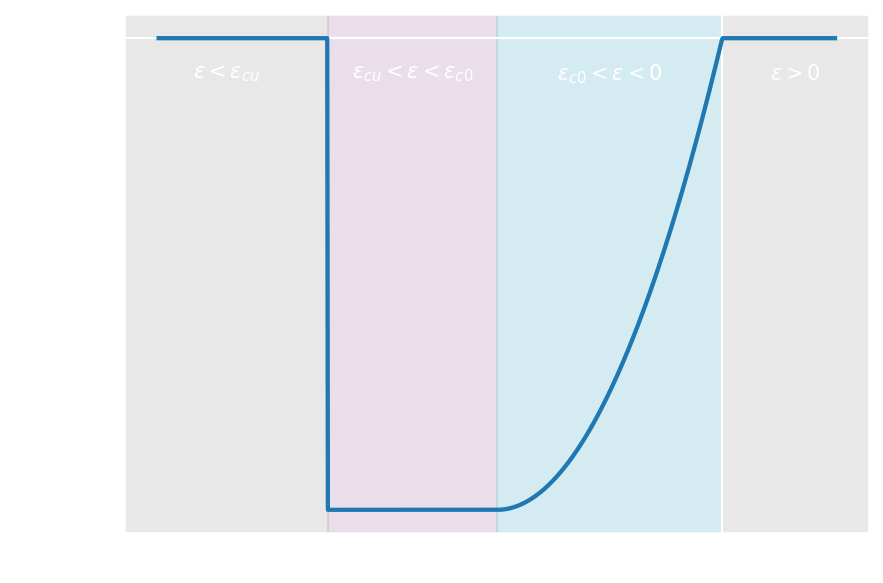
Parabola rectangle law.
The constitutive law can therefore be written as:
Substituting (10) in (18) the Marin coefficients for each branch can be determined. They are reported in the following table.
Branch name |
Strain range |
\(a_0\) |
\(a_1\) |
\(a_2\) |
|---|---|---|---|---|
Parabolic portion |
\(\varepsilon_{c0} \le \varepsilon < 0\) |
\(\dfrac{f_c \varepsilon_{0}}{\varepsilon_{c0}} \left( 2 - \dfrac{\varepsilon_0}{\varepsilon_{c0}} \right)\) |
\(\dfrac{2 f_c \chi_y}{\varepsilon_{c0}} \left( 1 - \dfrac{\varepsilon_0}{\varepsilon_{c0}} \right)\) |
\(- \dfrac{f_c \chi_y^2}{\varepsilon_{c0}}\) |
Constant portion |
\(\varepsilon_{cu} \le \varepsilon < \varepsilon_{c0}\) |
\(f_c\) |
n.a. |
n.a. |
Zero |
otherwise |
0.0 |
n.a. |
n.a. |
The __marin__ method return the coefficients reported in the table above and the strain limits for each portion.
Then the integrator discretizes the polygon cutting it into the portions needed (depending on the strain distribution in the polygon) and for each subpolygon the exact Marin integration is performed.
If the function to be integrated over the cross-section is the stiffness, represented by the following function (only corresponding to the parabolic portion, being 0 elsewhere):
one can write the stiffness as a function of \(z\):
The marin coefficients for stiffness function integration are therefore:
Branch name |
Strain range |
\(a_0\) |
\(a_1\) |
|---|---|---|---|
Parabolic portion |
\(\varepsilon_{c0} \le \varepsilon < 0\) |
\(\dfrac{2 f_c}{\varepsilon_{c0}} \left( 1 - \dfrac{\varepsilon_0}{\varepsilon_{c0}}\right)\) |
\(- \dfrac{2 f_c}{\varepsilon_{c0}} \dfrac{\chi_y}{\varepsilon_{c0}}\) |
Zero |
otherwise |
0.0 |
n.a. |
UserDefined constitutive law
A UserDefined constitutive law (see api documentation) permits the user to input any custom law discretizing it in a piecewise linear function.
In this case, for each branch, the __marin__ function return the coefficients \(a_0\), \(a_1\) and the strain limits for the branch.
Then the integrator discretizes the polygon cutting it into how many portions needed for the several branches (depending on the strain distribution in the polygon) and for each subpolygon the exact Marin integration is performed
For each \(i\)-th branch, the constitutive law can be written as:
And substituting (10) in (21), the stress function can be written as:
Having introduced the symbol \(K_i\) for the stiffness of the \(i\)-th branch.
Therefore the Marin coefficients \(a_n\) for each branch of a piecewise-linear elastic material are:
The Marin coefficient for stiffness function integration for each branch of a piecewise-linear elastic material is: